That Computes

Performance management comprises three sequential processes: monitoring, analysis, and modeling (Figure 1). Monitoring is the theme of this article, analysis is the ability to identify patterns in monitored data, and modeling uses monitored data to predict future events, such as resource bottlenecks. PDQ (Pretty Damn Quick), a queuing analysis tool that comes as a Perl module, helps make predictions possible.

Introduction

Choosing a monitoring solution and completing the installation and configuration isn't the end; it's just a new starting point. The core requirement is to collect monitored performance data. Without that, the performance characteristics of systems and applications cannot begin to be quantified. That is the monitoring phase.

But, monitoring alone is akin to watching needles jitter on the dashboard of a car or the cockpit of an aircraft. To assess the future picture, it is important to look out the window and see what is down the road or what other aircraft might be flying near you. The problem with just relying on monitoring alone is that it only provides a short-term view of system behavior (Figure 2). Looking out the window provides the longer range view, but the further away things are, the more difficult it is to discern their importance.

Additionally, the monitored performance data needs to be time-stamped and stored in a database. The next phase, performance analysis, builds on this by putting the administrator in a position to consider the collected data from a historical perspective and identify patterns and trends in the data.

The performance prediction phase builds on performance modeling and puts the administrator in a position to look out the window and into the future. To do so, you need additional tools that process the data so it can flow into performance models, and this involves some math.

Statistics vs. Queues

There are two classical approaches to performance modeling: statistical data analysis and the queuing model. Although these methodologies are not mutually exclusive, the distinction between them can be summarized as follows: Statistical data analysis, a task common in every accounting department, is based on modeling trends in the raw data. Many clever techniques and tools have been developed by statisticians over the years, and much of this intelligence is available in open source statistical modeling packages like R [2].

The limitation of this approach, however, is that it is based solely on existing data. If the future holds some (pleasant or unpleasant) surprises that were not somehow foretold in the current data, the forecast will be unreliable. Those who play the stock market know that this happens all the time.

Queuing models, on the other hand, are not subject to these limitations because they, by definition, require that an abstraction of the real system be constructed using the queuing paradigm. The trade-off is that this typically involves more work than just doing trend analysis on raw data, and it assumes that the queuing abstraction is a faithful representation of the real system. To the degree that it is not, its predictions will also be unreliable. As I attempt to show in this article, constructing queuing models is nowhere near as difficult as it might seem from this comparison. In fact, it is often stunningly simple.

Roadmap

Initially, I will investigate queuing concepts based on the familiar example of cashier queues in the supermarket. Then, I will extend the fundamental concept to predict the scalability of a three-tier e-commerce application. At the end of the article, I will introduce realistic extensions to the performance models presented here and offer some guidelines for building predictive performance models. All of the examples use Perl and the PDQ open source queuing analysis tool, which I co-maintain with Peter Harding [3].

Why Queues?

Buffers and stacks are ubiquitous forms of storage in computer systems and communication networks. A buffer is a type of queue in which the order of arrival dictates the processing order. This is called FIFO (first in, first out) or FCFS (first come, first served). In contrast, a stack processes requests in LIFO (last in, first out) order, or if you prefer, LCFS (last come, first served). On Linux, the shell history buffer is a well-known queue. Like any physical implementation, it is generally constrained to a finite amount of storage space (the capacity). In theory, the queue can have unlimited capacity, as is the case with PDQ.

The queue is a good abstraction for shared use of resources. A familiar example is the checkout stand at a grocery store. This resource comprises requests for service (the people standing in line) and a service center (the cashier). When you finish your shopping, you want to leave the store as quickly as possible – this is the performance goal. That goal translates to spending the least time getting through checkout, technically known as the residence time (R).

Once a customer has decided on a specific checkout isle and joins the queue, the residence time is made up of two components: the time the customer spends waiting in line before they reach the cashier and the time they spend being served while the employee scans purchases, takes the payment, and hands out the change and receipt.

If you assume everybody waiting in line has more or less the same number of items in their shopping basket, you can expect the service times for each customer to average out to a similar value. Moreover, the length of the queue is directly related to the number of customers waiting. If the store is almost empty, the average wait time will be much shorter than at busy times.

The queue abstraction (Figure 3) offers a powerful paradigm for characterizing the performance of computer systems and networks, among other things, because they tie together the otherwise disparate performance metrics that are measured by monitoring tools.

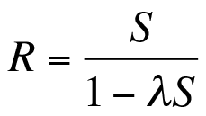
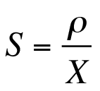
In this article, I continually refer to the metrics in Table 1 and, more specifically, to the relationship between the residence time (R), the service time (S), and the arrival rate (lamba), as shown in Equation (1).

(1)

You can view Equation (1) as a very simple performance model. The input for the model is on the right; the output on the left. Computations with PDQ use exactly the same scheme. With this simple model, you can see immediately that, if you have a small number of shoppers, the time required to pass through checkout (the residence time) is identical to the service time. If no other shoppers arrive (lambda = 0), you can ignore everything except the time needed to scan a purchase and complete the payment.

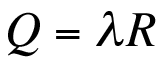
If the store is busy, such that the product lambdaS -> 1, the residence time also increases rapidly because the length of the queue is computed on the basis of the equation:

(2)

In other words, the residence time is directly related to the queue length by the arrival rate and vice versa.

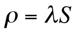
Equation (2) shows the relationship to monitored data. The load-averaged data shown in Figure 2 are instantaneous values sampled over relatively short time intervals (e.g., 1 minute). In contrast, the queue length (Q) is time-averaged over the entire measurement period of 24 hours. More intuitively, Q corresponds to the height of an imaginary rectangle that has the same area as that under the monitored data curve over the same 24-hour period. An analogous relationship also holds if the waiting is excluded from the residence time (R) in Equation (2) to get Equation (3).

(3)

In other words, if you replace R by the service time S on the right-hand side of Equation (2), the output volume on the left-hand side is equal to the utilization (rho).

In the late 1970s and early 1980s, several new theoretical developments led to simplified algorithms for computing the performance metrics of queuing circuits, and it is these algorithms that are incorporated into tools like PDQ. The latest developments in queuing theory have to do with modeling so-called self-similar or fractalized packet traffic on the Internet. Although these concepts lie well beyond the scope of this article, you can find this information elsewhere [4].

Assumptions in PDQ Models

One of the underlying assumptions in PDQ is that the average duration between arrivals and the average duration of service periods are both statistically randomized. Mathematically, this means that each arrival and service event belongs to a Poisson process. Then, the durations correspond to the average or mean of a negative Exponential probability distribution. Erlang discovered that traffic on the phone network conforms to this requirement. Methods are available for you to discover how well your monitored data conforms to this requirement [5].

If your monitored data differs very significantly from the Exponential requirement, it might be more prudent to resort to an event-based simulator (e.g., SimPy [6]), which is able to accommodate a broader class of probability distributions. The trade-off is that this takes longer to set up and debug (all simulation is about programming), and it takes longer to validate that your simulation results are statistically valid.

Another aspect that often bothers people about any kind of prediction is the errors introduced by the modeling assumptions. Although it is true that modeling assumptions introduce systematic errors into predictions and, thus, all PDQ results should really be presented as a range of plausible values with their attendant errors. What is often not appreciated is that everything that is quantified introduces errors – including monitored data. Contrary to popular opinion, data is not divine. Do you know the error range of your data?

Because all PDQ performance inputs and outputs are averages, it is important to ensure that monitored data also represents reliable averages. One way to do this is with a controlled load-test platform (Figure 4).

Such a platform is actually a workload simulator, and it is therefore important that all performance measurements be collected in steady state. A steady-state average throughput (X) for a given user load (N) is found by taking measurements over some lengthy measurement period (T) and eliminating any ramp-up or ramp-down periods from the data.

A nominal T might be on the order of 5 to 10 minutes, depending on the application. Industry standard benchmarks, such as those designed by SPEC [7] and TPC [8], have a requirement that all reported throughput results be measured in steady state.

A Simple Queue in PDQ

The relationship between the grocery store scenario and PDQ functions is summarized in Table 2.

On the basis of this approach, you can easily construct a simple model of a grocery store checkout – as Listing 1 for the Perl variant of PDQ shows. The PDQ code contains the input values for the arrival rate (lambda) and the service time (S):

01 #! /usr/bin/perl
02 # groxq.pl
03 use pdq;
04 #--------------- INPUTS ---------------
05 $ArrivalRate = 3/4; # customers per second
06 $ServiceRate = 1.0; # customers per second
07 $SeviceTime = 1/$ServiceRate;
08 $ServerName = "Cashier";
09 $Workload = "Customers";
10 #------------ PDQ Model ------------
11 # Initialize internal PDQ variable
12 pdq::Init("Grocery Store Checkout");
13 # Modify the units used by PDQ::Report()
14 pdq::SetWUnit("Cust");
15 pdq::SetTUnit("Sec");
16 # Create a PDQ control node (Cashier)
17 $pdq::nodes = pdq::CreateNode($ServerName, $pdq::CEN, $pdq::FCFS);
18 # Define the PDQ task and arrival rate
19 $pdq::streams = pdq::CreateOpen($Workload, $ArrivalRate);
20 # Define the service rate for customers at the cash desk
21 pdq::SetDemand($ServerName, $Workload, $SeviceTime);
22 #--------------- OUTPUTS ---------------
23 # Solve the PDQ model
24 pdq::Solve($pdq::CANON);
25 pdq::Report(); # generate a full PDQ report

(4)

(5)

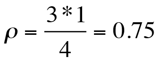
If you now apply the metric relations of Equation (2), cashier utilization is given by:

(6)

Similarly, using metric relations in Equations (1) and (2), the residence time output is given by

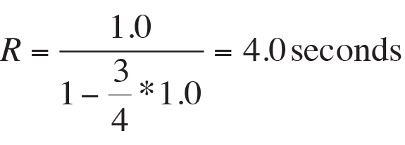(7)

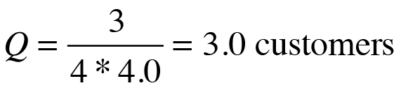
which states that the time spent at the checkout stand is equivalent to four average service periods when the cashier is 75 percent busy. The corresponding average queue length is:

(8)

For brevity, I only show the output portion of the generic PDQ report for this model (Listing 2). The computed PDQ values are identical to the theoretical predictions for throughput (X = lambda), utilization (rho), queue length (Q), and residence time (R).

01 *************************************
02 ***** Pretty Damn Quick REPORT ******
03 *************************************
04 *** of : Sun Feb 4 17:25:39 2007 ***
05 *** for: Grocery Store Checkout ***
06 *** Ver: PDQ Analyzer v3.0 111904 ***
07 *************************************
08 ****** RESOURCE Performance *******
09
10 Metric Resource Work Value Unit
11 --------- ------ ---- ----- ----
12 Throughput Cashier Customers 0.7500 Cust/Sec
13 Utilization Cashier Customers 75.0000 Percent
14 Queue Length Cashier Customers 3.0000 Cust
15 Residence Time Cashier Customers 4.0000 Sec
16 N Sws Sas Sdb
17 1 0.0088 0.0021 0.0019
18 2 0.0085 0.0033 0.0012
19 4 0.0087 0.0045 0.0007
20 7 0.0095 0.0034 0.0005
21 10 0.0097 0.0022 0.0006
22 20 0.0103 0.0010 0.0006
23 Avg 0.0093 0.0028 0.0009

Now that you are familiar with the fundamental terms and I have introduced PDQ as a tool for these computations, you can start applying these tools to problems, such as predicting the performance of individual hardware resources, such as the CPU execution speed [5] or the speed of a hard disk device drive. Most textbooks on queuing theory contain examples of this caliber, but to predict the performance of real systems, you must be able to simulate the workflow between multiple queues – that is, the interaction between requests issued to the CPUs, hard disks, and network at the same time. Next, I will show you how to fulfill this task using PDQ. (Open source load and stress test tools are available from opensourcetesting.org [9].)

Circuits of Queues

Requests that flow from one queue to another correspond to a circuit or network of queues. When only the arrival rate (lambda) of the requests, rather than the number of requesters, is monitored, it is referred to as an open circuit (Figure 5). An example of a situation of this kind that does not originate in the computing universe, is boarding a plane at an airport. The three stages are: waiting at the gate, queuing the jetway to get onto the aircraft, and finally queuing in the cabin aisle while passengers ahead of you are seated. The average response time (R) is given by the total time spent in each queuing stage, or the sum of the three residence times. In a computing context, you could apply this to a three-tier web application for which you only know the HTTP request rate.

Another form of queuing circuit involves a finite number (N) of customers or requests. This is precisely the situation created by a load-test platform. A finite number of load generators issues requests to the test rig, and no additional requests can enter the isolated system from external sources. Moreover, a kind of feedback mechanism takes effect here, in that no more than one request can be outstanding at a time. In other words, the script running on a load generator (e.g., a PC) does not issue the next measured request until the previous one has completed. This is known as a closed queuing circuit.

E-Commerce Application in PDQ

In this section, I show how you can apply the PDQ model of the closed system in Figure 6 to predict the throughput performance of the three-tier e-commerce application of the type shown in Figure 7. Because of the huge expense of an installation of this kind, load tests with a smaller model of the production environment are typical. In this example, each tier is represented by a single server. Such a test rig can provide an excellent platform for generating steady-state performance measurements that are useful for parameterizing a PDQ model. The throughput is measured in HTTP Gets per second (GPS), and the corresponding response times are measured in seconds (s).

Because of space limitations, I will focus entirely on simulating the throughput performance. If you are interested in the response times, you will find details of them elsewhere [5]. The key load-test measurements for this example are summarized in Table 3.

Unfortunately, the data is not presented in equal user-load increments, which is less than ideal for proper performance analysis but is not an insurmountable problem. X and R are system metrics reported from the client side. The utilization was obtained separately from performance monitors on each of the local servers. The monitored utilizations (rho) and throughputs (X) in Table 3 can be used together with a rearranged version of Equation (3) to ascertain the corresponding service times for each tier (Equation (9)). The service times for each load are summarized in Table 4.

Next, I show how the mean value of the measured service times (the last line in Table 4) can be used to parameterize the PDQ model.

(9)

Naive PDQ Model

A first attempt to simulate the performance characteristics of the e-business application in Figure 6 simply represents each application service as a separate PDQ node with the respective service demand determined from Table 4. In Perl::PDQ, the queue node is parameterized as in Listing 3.

01 #! /usr/bin/perl
02 # ebiz_final.pl
03 use pdq;
04 use constant MAXDUMMIES => 12;
05
06 # Hash AV pairs: (load in vusers, throughput in gets/sec)
07 %tpdata = ( (1,24), (2,48), (4,85), (7,100), (10,99), (20,94) );
08
09 @vusers = keys(%tpdata);
10 $model = "e-Commerce Final Model";
11 $work = "ebiz-tx";
12 $node1 = "WebServer";
13 $node2 = "AppServer";
14 $node3 = "DBMServer";
15 $think = 0.0 * 1e-3; # as per test system
16 $dtime = 2.2 * 1e-3; # dummy service time
17
18 # Header for user-specific report
19 printf("%2s\t%4s\t%4s\tD=%2d\n", "N", "Xdat", "Xpdq", MAXDUMMIES);
20
21 foreach $users (sort {$a <=> $b} @vusers) {
22 pdq::Init($model);
23 $pdq::streams = pdq::CreateClosed($work, $pdq::TERM, $users, $think);
24 $pdq::nodes = pdq::CreateNode($node1, $pdq::CEN, $pdq::FCFS);
25 $pdq::nodes = pdq::CreateNode($node2, $pdq::CEN, $pdq::FCFS);
26 $pdq::nodes = pdq::CreateNode($node3, $pdq::CEN, $pdq::FCFS);
27
28 # Time basis in seconds " expressed in milliseconds
29 pdq::SetDemand($node1, $work, 8.0 * 1e-3 * ($users ** 0.085));
30 pdq::SetDemand($node2, $work, 2.8 * 1e-3);
31 pdq::SetDemand($node3, $work, 0.9 * 1e-3);
32
33 # Create dummy node with corresponding service times ...
34 for ($i = 0; $i < MAXDUMMIES; $i++) {
35 $dnode = "Dummy" . ($i < 10 ? "0$i" : "$i");
36 $pdq::nodes = pdq::CreateNode($dnode, $pdq::CEN, $pdq::FCFS);
37 pdq::SetDemand($dnode, $work, $dtime);
38 }
39
40 pdq::Solve($pdq::EXACT);
41 printf("%2d\t%2d\t%4.2f\n", $users, $tpdata{$users},
42 pdq::GetThruput($pdq::TERM, $work));
43 }

A plot of the predicted throughput in Figure 8 shows that the naive PDQ model has a throughput that saturates too quickly when compared with the test rig data. However, PDQ also tells you that, given the measured service times in Table 4, the best possible throughput for this system is about 100GPS.

This performance is caused by a resource bottleneck (the queue with the longest average service time), which is the front-end web server in this example. It constrains the throughput in such a way that the maximum throughput cannot exceed the value resulting from the relation in Equation 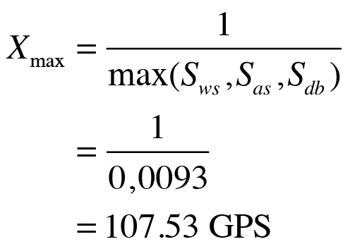(10).

(10)

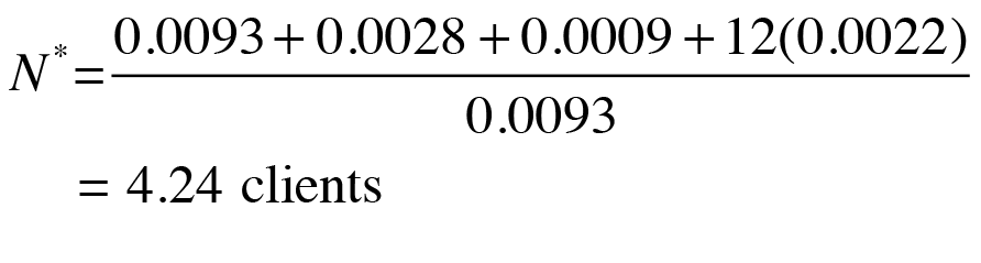
The highest possible throughput, as you can see in Equation (11), is achieved in close proximity to the computed optimum load point N^*,

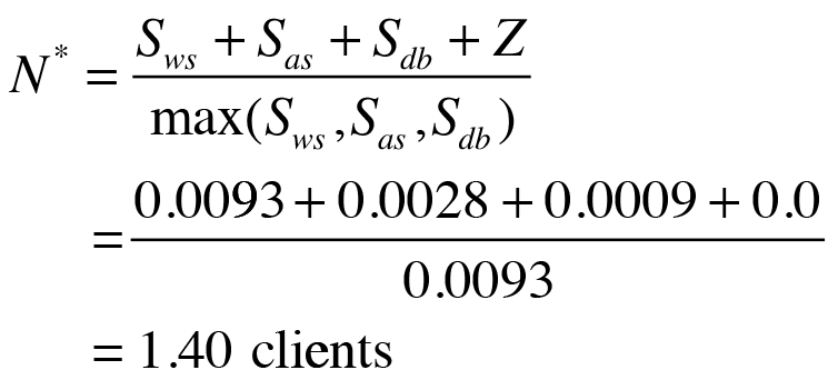(11)

which is 1.40 clients, not 20 clients. If the service times change in the future (e.g., for a new release of the application), the resource bottleneck might change, and the PDQ model will be able to predict its effect on throughput and response times.

Clearly then, it is also desirable to model the overall data set better than the naive PDQ model has achieved so far. One simple method to offset this rapid saturation in the throughput is to introduce a non-zero value to the think time of Z > 0 (Figure 9):

$think = 28.0 * 1e-3; # free parameter
...
pdq::Init($model);
$pdq::streams = pdq::CreateClosed($work, $pdq::TERM, $users, $think);

This has the effect of reducing the speed at which new requests are injected into the system. In this sense, you can play with the think time as if were a free parameter. The non-zero Z = 0.028 seconds disagrees with the settings in the load-test scripts, but it can give you an idea in which direction you have to work to improve the PDQ model. As Figure 9 shows, a non-zero think time improves the throughput profile quite dramatically.

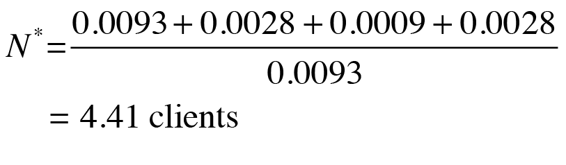(12)

This trick with the think time reveals the existence of other latencies that were not accounted for in the load-test measurements. The effect of the non-zero think time is to add latency and make the round trip time of a request longer than anticipated. This also has the effect of reducing the throughput at low loads. But the think time was set to zero in the actual measurements. How can this paradox be resolved?

Allowing for Hidden Latencies

The next trick is to add dummy nodes to the PDQ model (Figure 10). However, the service requests of the virtual nodes need to fulfill certain conditions. The service demand of each dummy node must be chosen in such a way that it does not exceed the service demand of the bottleneck node. Additionally, the number of dummy nodes must be chosen such that the sum of their respective service demands does not exceed R_min = R₍₁₎ if no competition occurs (i.e., for a single request). It turns out that these conditions can be fulfilled by introducing 12 uniform dummy nodes, each with a service demand of 2.2ms. The change to the relevant PDQ code fragment is:

use constant MAXDUMMIES => 12;
$think = 0.0 * 1e-3; #same as in test rig
$dtime = 2.2 * 1e-3; #dummy service time
# Create dummy nodes with service times
for ($i = 0; $i < MAXDUMMIES; $i++) {
     $dnode = "Dummy" . ($i < 10 ? "0$i" : "$i");
     $pdq::nodes = pdq::CreateNode($dnode, $pdq::CEN, $pdq::FCFS);
     pdq::SetDemand($dnode, $work, $dtime);
}

Notice that the think time is now set back to zero. The results of this change to the PDQ model are shown in Figure 11. The throughput profile still maintains a good fit at low loads (N < N^*), where

(13)

but needs improvement above N^*.

Load-Dependent Server

Certain aspects of the physical system were not measured, and this makes PDQ model validation difficult. Thus far, I have attempted to modify the intensity of the workload by introducing a positive think time. Setting Z = 0.028 seconds removed the rapid saturation but is inconsistent with Z = 0 seconds that was set for the test measurements.

Introducing the dummy queuing nodes into the PDQ model improved the low-load model, but it does not accommodate the throughput roll-off observed in the data. To model this effect, you can replace the web server node with a load-dependent node. The general theory behind load-dependent servers is discussed in Analyzing Computer System Performance with Perl::PDQ [5]. In the example shown here, I apply a slightly more simple approach. The service time (S_ws) in Table 4 indicates that it is not constant across all client loads. In other words, you need a way to express this variability. If you plot the monitored data for Sws, you can fit the statistical regression, as shown in Figure 12.

The resulting power law equation is given by:

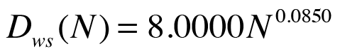(14)

Thus, node 1 in the PDQ model is parameterized as follows:

pdq::SetDemand($node1, $work, 8.0 * 1e-3 * ($users ** 0.085));

The customized output of the complete PDQ model is shown in Table 5. It demonstrates good agreement with the measured data for D = 12 dummy PDQ nodes.

The effect on the throughput model can be gauged from Figure 13. The curve labeled Xpdq2 is the predicted overdriven throughput based on the load-dependent server for the web front end, and the predictions fit well within the error margins of the measured data.

In this case, there is little virtue in using PDQ to project beyond the measured load of N = 20 clients because the throughput is not only saturated, it is also retrograde. However, now that a PDQ model has been constructed and validated against test data, it can be used to address any number of what if scenarios.

The previous example is fairly sophisticated, and similar PDQ models are typically fine for most applications; but in some cases, a detailed model can be necessary. Two examples of this scenario are multiple servers and multiple workloads.

Multiple Servers

A scenario outside of the computing universe that you can simulate as a queue with multiple servers, as shown in Figure 14, is standing in line at a bank or post office. In the context of computer performance, Figure 14 could be used as a simple model of a symmetric multiprocessor [5].

The response time in Equation (1) is replaced by

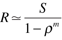(15)

where rho = lambdaS and m is the integral number of servers. From a technical point of view, this is an approximation, but not a bad one. The exact solution is more complex and can be found using the Perl algorithm in Listing 4. This is precisely the queuing model developed by Erlang 100 years ago. In that case, each server represented a trunk telephone line.

01 #! /usr/bin/perl
02 # erlang.pl
03
04 ## Input-Parameter
05 $servers = 8;
06 $erlangs = 4;
07
08 if($erlangs > $servers) {
09 print "Error: Erlangs exceeds servers\n";
10 exit;
11 }
12
13 $rho = $erlangs / $servers;
14 $erlangB = $erlangs / (1 + $erlangs);
15
16 for ($m = 2; $m <= $servers; $m++) {
17 $eb = $erlangB;
18 $erlangB = $eb * $erlangs / ($m + ($eb * $erlangs));
19 }
20
21 ## Output the results
22 $erlangC = $erlangB / (1 - $rho + ($rho * $erlangB));
23 $normdwtE = $erlangC / ($servers * (1 - $rho));
24 $normdrtE = 1 + $normdwtE; # Exact
25 $normdrtA = 1 / (1 - $rho**$servers); # ca.

Multiple Workloads

What often happens in real life is that a single resource, such as a database server, has to handle a multitude of transaction types. For example, booking a flight or a hotel room on the Internet can require half a dozen different transactions before you get your confirmation number or finally book the room. Situations of this type can be simulated in PDQ.

In a simpler case, consider three different transaction types represented by the colors red, green, and blue. Each of these colored workloads may access a common resource (e.g., a database server). In the queuing paradigm (Figure 15), each of these colored workloads is distinguished by their different service time requirements when they get serviced.

In other words, the red work takes a red service period, the green work takes a green service period, and so on. Each color has its own arrival rate as well. If you assume that the service times differ, the real effect of a red request reaching the queue is not a product of the number of requests already waiting in the queue, its response time will be determined not by the number of requests ahead of it (which is only true for a "monochromatic" workload), but by the particular combination of colors ahead of it. In PDQ, you could represent Figure 15 as in Listing 5.

01 $pdq::nodes = pdq::CreateNode("DBserver", $pdq::CEN, $pdq::FCFS);
02 $pdq::streams = pdq::CreateOpen("Red", $ArrivalsRed);
03 $pdq::streams = pdq::CreateOpen("Grn", $ArrivalsGrn);
04 $pdq::streams = pdq::CreateOpen("Blu", $ArrivalsBlu);
05 pdq::SetDemand("DBserver", "Red", $ServiceRed);
06 pdq::SetDemand("DBserver", "Grn", $ServiceGrn);
07 pdq::SetDemand("DBserver", "Blu", $ServiceBlu);

Naturally, the PDQ report generated by multiple workloads will be more complicated because of all the possible interactions, but it gives some idea of the ways in which PDQ can be extended to reflect more realistic computer architectures. Further discussion of these matters is beyond the scope of this article, but interested readers can find more details in my book [5].

Guidelines for Applying PDQ

Performance modeling of any type is part science and part art. Thus, it is impossible to provide a complete set of rules or algorithms that will furnish the correct model. In fact, as shown here, the process is one of iterative improvement. The best guide is experience, and experience comes from simply doing something repeatedly. With this in mind, I'll give you a few guidelines that might help you construct PDQ models.

Keep it simple. A PDQ model should be as simple as possible, but no simpler! It is almost axiomatic that the more you know about a system architecture, the more detail you will try to throw into the PDQ model. However, if you do so, you will inevitably overload the model.

Keep the map, not the metro, in mind. A PDQ model is to a computer what a map of a subway system is to the underground railway network. A subway map is an abstraction that has very little to do with the physical characteristics of the network. It encodes only sufficient detail to enable you to transit from point A to point B. It does not include a lot of irrelevant details such as altitude of the stations, or even their actual geographical proximity. A PDQ model is a similar kind of abstraction.

Mind the big picture. Unlike most aspects of computer technology, which require you to absorb large amounts of minute detail, PDQ modeling is all about deciding how much detail can be ignored!

Seek the operative principle. If you cannot describe the principle of operation in fewer than 25 words, you probably do not understand it well enough to start constructing a PDQ model. The principle of operation for a time-share computer system, for example, can be stated as: Time sharing gives every user the illusion that they are the only active user on the system. The hundreds of lines of code in Linux to implement time-slicing, priority queues, and so on are there merely to support this illusion.

Guilt is golden. PDQ modeling is also about spreading the guilt around. You, as the performance analyst, only have to shine the light on the performance problem, then stand back while others flock to fix it.

Choose where to start. One place to start constructing a PDQ model is by drawing a functional block diagram. The objective is to identify where time is spent at each stage in processing the workload of interest. Ultimately, each functional block gets converted to a queuing subsystem. This includes the ability to distinguish sequential and parallel processing. Other diagrammatic techniques (e.g., UML diagrams) could also be useful.

Know your inputs and outputs. When defining a PDQ model, it is useful to create a list of inputs (measurements or estimates used to parameterize the model) and outputs (numbers generated by calculating the model).

No service, no queues. You know the restaurant rule: "No shoes, no service!" Well, the PDQ modeling rule is: No service, no queues. In a PDQ model, it makes no sense to create more queuing nodes than those for which you have measured service times. If the measurements of the real system do not include the service time for a PDQ node that you think ought to be in your model, then that PDQ node cannot be defined.

Estimate the service times. Service times are notoriously difficult to measure directly. Often, however, the service time can be calculated from other performance metrics that are easier to measure (see Table 3).

Change the data. If the measurements don't support the PDQ performance model, you probably need to repeat the measurements.

Open or closed queue? When deciding which queuing model to apply, ask yourself whether you have a finite number of requests to service. If the answer is "yes" (as it should be for a load-test platform), then it is a closed queuing model; otherwise, use an open queuing model.

Take measurements in steady state. The steady-state measurement period should be on the order of 100 times larger than the largest service time.

Use an appropriate time base. Use the time base of your measurement tools. If the tool reports in seconds, use seconds; if it reports in microseconds, use microseconds. In the case of multiple monitoring sources of data, all numbers should be normalized to the same units before doing any calculations.

Workloads come in threes. In a mixed-workload model (multiclass streams in PDQ), avoid more than three concurrent work streams if possible. Apart from generating a PDQ report that is unwieldy to read, generally you are only interested in the interaction of two workloads – that is, a pairwise comparison. Everything else is part of the third workload (the "background"). If you cannot see how to do this, you are probably not ready to create the PDQ model.

Conclusions

Performance modeling is a complex discipline that is best learned by constant practice. Much of the effort is concentrated in creating and validating a model of the environment under investigation and its applications. Once you have validated the PDQ model, there is no need to keep reconstructing it. Generally speaking, a bit of tuning will suffice.

The three-tier e-commerce application used as the sample model for this article is a pretty good starting point on which to build. You can extend the model to consider multiple servers and additional tasks fairly simply. One of the most surprising results of the PDQ model is that it lets the administrator performing the analysis identify certain effects – for example, hidden latencies – that would otherwise have remained invisible in the monitoring data. Perhaps one of the most important outcomes of using PDQ is not the models per se, but that it provides an organizational framework in which to understand performance data from monitoring to prediction.