On Track

Large volumes of data are most useful if you can study them with intensive data analysis. The open source language, R [1], is a powerful tool for evaluating an existing database. The R language offers a variety of statistical functions, but R can do more.

This article shows how to use R for a sample application that evaluates comet data. An Apache web server visualizes the results of statistical reports – with the help of web technologies such as HTML, JavaScript, jQuery [3], and CSS3, which Python creates in combination with R and the MongoDB [4] database.

Comet Rising

Figure 1 shows how the report generator of the sample application displays the comet data in Firefox. The selection list at the top lets the user select a report variant. If you click on Send, JavaScript sends an HTTP request to the Apache web server, which then generates the report.

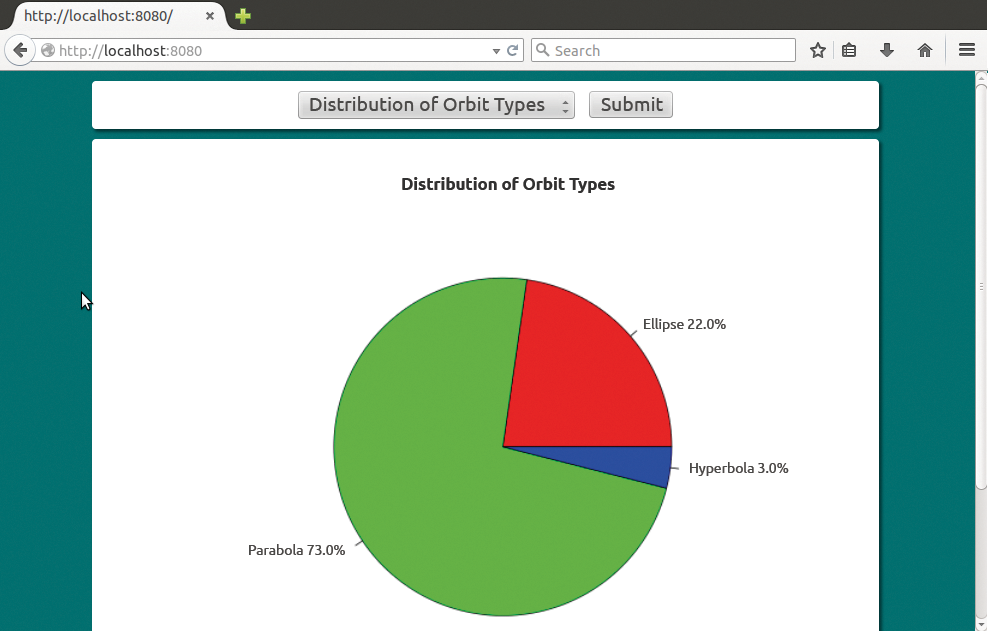
The Python scripts first save the comet data in a MongoDB database. Scripts then parse the data and draw on R to create the report in the form of a graphic, which ends up as a PNG file in a public directory on the web server. The server sends the URL back to the browser as a response to the HTTP request.

Web Server

Using the instructions in Listing 1, the developer first prepares the Apache web server on Ubuntu 12.04 for running the sample application. The web server copies the script from the listing (with root privileges) to the /etc/apache2/site-available/rconf path. The command sudo a2ensite binds it into the web server's configuration; sudo service apache restart enables the extended configuration by restarting the web server.

01   Listen 8080
02   <VirtualHost *:8080>
03    DocumentRoot /home/pa/www
04    <Directory /home/pa/www>
05     Options +ExecCGI
06     AddHandler cgi-script .py
07    </Directory>
08   </VirtualHost>

Users can then access the sample application via the URL http://localhost:8080. Line 1 tells Apache to listen on port 8080; lines 2 to 8 handle the incoming HTTP requests. Lines 5 and 6 allow Python scripts to execute via the web server's CGI interface, assuming they reside in the /home/pa/www root directory.

Data Store

The sample application uses the free NoSQL, MongoDB [4] database system as its data repository. The commands from Listing 2 install the current version 2.6.2 on Ubuntu 12.04. Line 1 retrieves the keys for the external repository, and line 2 integrates the key. Line 3 updates the package list. The last two lines install mongodb-org and the current version of the Python Pymongo interface.

01 sudo apt-key adv --keyserver hkp://keyserver.ubuntu.com:80 --recv 7F0CEB10
02 echo 'deb http://downloads-distro.mongodb.org/repo/ubuntu-upstart dist \
   10gen' | sudo tee /etc/apt/sources.list.d/mongodb.list
03 sudo apt-get update
04 sudo apt-get install -y mongodb-org
05 sudo easy_install pymongo

To import the sample data into MongoDB, you need the Python import_comets.py script from Listing 3.

01 from pymongo import MongoClient
02 import csv
03 import sys
04
05 def pfl(val):
06   try:
07     return float(val)
08   except:
09     return None
10
11 with open(sys.argv[1]) as csvfile:
12   collec = MongoClient()["galaxy"]["comets"]
13   for row in csv.reader(csvfile, delimiter="\t"):
14     try:
15       collec.insert({"name":row[0],"observer":row[1],"type":row[2],"period":\
         pfl(row[3]), "ecc":pfl(row[4]),"semaj_axs":pfl(row[5]), \
         "perih_dist":pfl(row[6]), "incl":pfl(row[7]), "abs_mag":pfl(row[8])})
16     except:
17       print "Error: could not import: ", row

The python import_comets.py data/comets.csv command starts the import at the command line. The script then parses the sample data from the CSV file, data/comets.csv.

Line 1 integrates MongoClient from the Python pymongo package; the next two lines import the csv and sys modules. Line 11 reads the CSV file path from the field in the sys.argv command-line parameter, opens the file, and stores the resulting descriptor in the csvfile variable.

If they do not already exist, the Python script then creates the MongoDB database galaxy and the comets data collection in line 12. The reader() method then parses the CSV file and splits it into columns based on the tab character.

The for loop fetches the next line from the reader object and stores it in the row field. Line 15 then finally stores the record from the row in the form of a Python dictionary with key/value pairs in the MongoDB database. The pfl() function converts numeric values to floating points. If the conversion fails, the script returns a value of None.

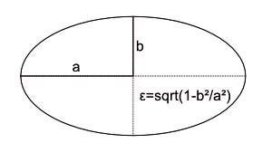
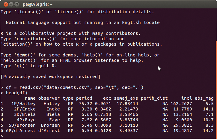
The keys match the attributes in Table 1. The sample data provides characteristic parameters for known comets. Comets primarily differ in terms of their trajectory shapes. Just like planets, comets move in repetitive elliptical orbits (Figure 2).

Results Oriented

R is a free implementation of the statistics programming languages S and S-Plus. Like the S languages, R facilitates the process of performing statistical computations and generating matching graphics (see the "Interactive R" box for more information). R is licensed under the GPL, and the current version is 3.1.2. Listing 4 shows the installation of the current version on Ubuntu 12.04.

sudo apt-key adv --keyserver keyserver.ubuntu.com --recv-keys E084DAB9
sudo add-apt-repository ppa:marutter/rrutter
sudo apt-get update
sudo apt-get install r-base r-base-dev

Like JavaScript, R exclusively stores values in objects, which it binds lexically to an environment or a closure object. The most commonly used data types are vectors, matrices, lists, and data frames. R processes the values with the help of various built-in function and operators, typical control structures, and user-defined functions and operators. The Comprehensive R Archive Network (Cran [5]) also offers many modules for R.

R Interface

The sample application uses the Python Rpy2 [6] package as an interface to R. Rpy2 passes in the data and function calls via R's C interface to an embedded R process and accepts the results. Rpy2 also provides an object-based interface to R in the form of the robjects module; it includes a separate Python class for each R object type.

The R functions work with the objects of the Python classes as they do with native R objects: For example, they convert the Python expression robjects.r. length(robjects.FloatVector([1.0, 2.0]) to the expression length(c(1.0, 2.0)) for the R process and evaluate it in the process. Rpy2 is licensed under the GPLv2 and is currently at version 2.5.4. Listing 5 installs the current version of Rpy2 on Ubuntu 12.04.

sudo apt-get install python-dev
sudo easy_install rpy2

Reports

The Python reports in the sample application all use the reporter class from Listing 6 (lines 5 to 21) to read data from the MongoDB database and convert it to a Python dataframe object with the help of R. Their constructor adds the name of a MongoDB database and a data collection, a list of attributes, and an optional selector in its list of parameters (line 6).

01 from pymongo import MongoClient
02 import rpy2.robjects as ro
03 import json
04
05 class reporter:
06   def __init__(self, name, collec, keys, fexpr=None):
07     count = 0
08     doc = None
09     for doc in MongoClient()[name][collec].find(fexpr):
10       try:
11         if count == 0:
12           ro.r('df = %s' %ro.Dataframe({key: float(doc[key]) for key in keys}).r_repr())
13           count += 1
14         else:
15           ro.r('df[nrow(df)+1,] = %s' %ro.FloatVector([float(doc[key]) for key in keys]).r_repr())
16       except:
17         pass
18     self.df = ro.r('df')
19
20   def respond(self, obj):
21     print "Content-Type: application/json;charset=utf-8\n\r\n\r%s" %json.dumps(obj)

Lines 9 through 18 iterate against all entries of a database cursor, which the call to the find() method in line 9, generates from the queried data collection.

During the first loop, the Dataframe constructor (line 12) generates an object from the dictionary passed into it. The generator expression creates the dictionary in the curly brackets from the list of attributes, the keys call parameter, and the keys attribute values from the current cursor entry from the doc variable. After instantiation, the r_repr() method converts the object into a string and replaces %s in df = %s with it.

The embedded R process evaluates the object as a dataframe object with the help of the r() method, finally saving it in the df variable. In a similar way, the second R side loop iteration in line 15 adds df to the cursor entries it reads. This time, the r() method dumps the values into a FloatVector type object and substitutes them into the R expression df[nrow(df)+1,] = %s.

Line 18 saves the dataframe created in this way as a Python object in the self.df component. The Python scripts use respond() as of line 20 to transfer the resulting URL to the web server like a CGI response. Line 21 appends the Python object to the header in JSON format.

Listing 7 generates the first report. The report shows the relative frequency of the ellipse, parabola, and hyperbola orbit types as a pie diagram (Figure 1). In the shebang (#!) line, the script first selects Python as the executing instance. The script uses the importr() method to retrofit R modules and then imports the reporter class from Listing 6 and the robjects module.

01 #!/usr/bin/env python
02 from rpy2.robjects.packages import importr
03 from rreport import reporter
04 import rpy2.robjects as ro
05
06 devs = importr('grDevices')
07
08 main = "Distribution of Orbit Types"
09 path = "tmp/bahntypen.png"
10
11 rep = reporter("galaxy", "comets", ["ecc"])
12 num = ro.r.nrow(rep.df)[0]
13 vals = ro.r.table(ro.r.cut(rep.df.rx2(1), [0, 0.9999, 1.0001, 2]))
14
15 label = lambda label, i: "%s %s %%" %(label, round((vals[i]*100)/num))
16 labels = [label("Ellipse", 0), label("Parabola", 1), label("Hyperbola", 2)]
17 col = ro.r.rainbow(len(labels))
18
19 devs.png(file=path, width=512, height=512)
20 ro.r.pie(vals, labels=labels, col=col, main=main)
21 devs.dev_off()
22
23 rep.respond({"fileref":path})

Line 6 uses importr() to integrate the export mechanism for graphs into the running R process. The main variable in line 8 stores the report title; the Python script uses path in line 9 to create the path for the graph to be created relative to its own storage location. Line 11 generates an object of the reporter class as an instance and stores it in the rep variable. The call to the constructor uses the MongoDB name (galaxy) and the data collection name (comets). The list in the third call parameter requests the eccentricity values.

Line 12 uses nrow to count the records in the dataframe object, rep.df, and stores the results in the num variable. The rx2() first copies the values from the first column of rep.df to a FloatVector type object. The cut() maps the vector components to one of the three R factors, [0-0.9999), [0.999-1.0001), or [1.0001-2) (these are semi-open intervals), and uses table() to create a contingency table from the resulting vector. The vals variable stores the table.

The lambda function in line 15 formats the pie labels using a designator in the label variable and an index in i. The function references i, vals, and num compute the relative frequency of the orbit type as a percentage.

By repeatedly calling the lambda function, line 16 generates and stores labels in the labels field; line 17 generates a color index for the pie segments in three colors. Line 19 uses png() to open the file from the path variable to store the figures. Line 20 uses pie() to create the pie chart.

The function imports the vals contingency table with the graphics options from lines 16, 17, and 18. Line 21 stops the output to the file before rep.respond() has sent the relative URL for the graph to the browser as an HTTP response.

The Kepler3.py report in Listing 8 verifies the validity of Kepler's third law [7], according to which the square of the orbit time T of a celestial body moving in an elliptical orbit about the sun is proportional to the cube of its semi-major axis: T^2 ~ a^3. If you plot a^3 vs. T^2, the result should be a straight line according to Kepler.

Listing 8 differs from Listing 7 as of line 11 in that it loads the values of the semi-major axis and the orbit time into the dataframe object. The last parameter in the constructor call in line 11 contains the MongoDB selector {"semaj_axs":{"$lt":100}}, which the reporter class from Listing 6 passes to the find() method. The selector only selects data from comets with a large half-axis of less than 100AU.

01 #!/usr/bin/env python
02 from rpy2.robjects.packages import importr
03 from rreport import reporter
04 import rpy2.robjects as ro
05
06 devs = importr('grDevices')
07
08 main = "3. Kepler's Law"
09 path = "tmp/Kepler3.png"
10
11 rep = reporter("galaxy", "comets", ["semaj_axs", "period"], {"semaj_axs":{"$lt":100}})
12 x_lab = "Semi-major axis / [AU]"
13 x_vals = ro.FloatVector([x**3 for x in rep.df.rx2(1)])
14
15 y_lab = "Orbital Period / [Years]"
16 y_vals = ro.FloatVector([x**2 for x in rep.df.rx2(2)])
17
18 devs.png(file=path, width=512, height=512)
19 ro.r.plot(x_vals, y_vals, xlab=x_lab, ylab=y_lab, main=main)
20 devs.dev_off()
21
22 rep.respond({"fileref":path})

In line 12, the variable x_lab stores the label for the x-axis. Line 13 accepts the generator expression with the values for the cube of the semi-major axis and passes the results on to the constructor of the FloatVector class, which stores them in the x_vals variable.

Lines 15 and 16 repeat the procedure for the orbit time and the y-axis. The plot() function creates a dot diagram, which plots x_vals vs. y_vals (Figure 5). The dots are in a straight line, as expected.

Listing 9 compares the distribution of the eccentricities for regular periodic comets ({"type":"RP}) with the normal distribution using a quantile-quantile plot qqnorm() (line 14). The call to qqline() retroactively draws a model straight line in the graph. The closer the quantile of the measure distribution matches that of the normal distribution, the closer the points are to the model straight line that halves the angle (Figure 6).

01 #!/usr/bin/env python
02
03 from rreport import reporter
04 from rpy2.robjects.packages import importr
05 import rpy2.robjects as ro
06
07 devs = importr('grDevices')
08
09 path = "tmp/qqnorm.png"
10
11 rep = reporter("galaxy", "comets", ["ecc"], {"type":"RP"})
12
13 devs.png(file=path, width=512, height=512)
14 ro.r.qqnorm(rep.df.rx2(1))
15 ro.r.qqline(rep.df.rx2(1))
16 devs.dev_off()
17
18 rep.respond({"fileref":path})

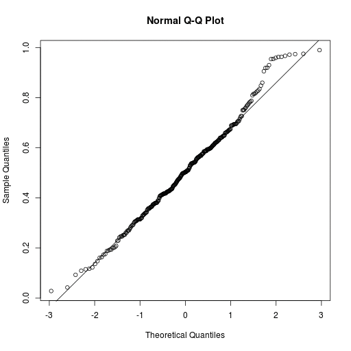
The distribution of the eccentricities is similar to the normal distribution for the most part but deviates too substantially from it for larger values. These comets might be subject to major scatter processes.

Web Interface

Listing 10 shows the HTML document for the sample application. The header binds the JavaScript jQuery library and the JavaScript code for generating reports into the CSS3 stylesheet. The selection list is generated by lines 12 to 16. The value attributes of the option elements store the respective URLs for the Python reports. Line 17 generates the Submit button. The div element, which contains id="output" (line 20), outputs the results.

01 <!DOCTYPE html>
02 <html>
03 <head>
04  <meta charset="UTF-8"/>
05  <link href="css/styles.css" rel="stylesheet"></link>
06  <script src="//ajax.googleapis.com/ajax/libs/jquery/2.1.1/jquery.min.js">\
    </script>
07  <script src="js/app.js"></script>
08 </head>
09 <body class="centered">
10  <div class="container">
11   <form>
12   <select id="report">
13    <option value="bahntypen.py">Distribution of Orbit Types</option>
14    <option value="Kepler3.py">3. Kepler's Law</option>
15    <option value="eccdistr.py">Distribution of Orbit Eccentricities</option>
16   </select>
17   <input type="submit" value="Submit"/>
18   </form>
19  </div>
20  <div id="output" class="container"><p>Please Select</p></div>
21 </body>
22 </html>

Listing 11 finally shows the JavaScript code that the jQuery expression in line 7 of Listing 10 integrates. The script initializes the JavaScript code after the browser has fully loaded the web page from Listing 10. The callback function in lines 2 to 8 is enabled on sending the form in Listing 10. The preventDefault() method first interrupts the transmission process before the following line uses the image() function to send a Loader image to the output area.

01 $(document).ready(function() {
02  $('form').submit(function(e) {
03   e.preventDefault();
04   image("/img/ajax-loader.gif");
05   $.getJSON($('#report').val(), function(data) {
06    image(data.fileref);
07   }).fail(function(e) {out($('<p>').text("Error: " + e.status + \
                                            " - " + e.statusText))});
08  });
09
10  function image(url) {
11   out($("<img>").attr("src", url+"?"+(Date.now())));
12  }
13
14  function out(obj) {
15   $('#output').empty().append(obj);
16  }
17 });

As of line 5, jQuery uses getJSON() to launch a report on the web server. getJSON() sends an asynchronous HTTP request to the web server and expects a document in JSON format in response.

jQuery uses $('#report').val() to read the URL for the HTTP request --from the value attribute of the currently selected item in the selection list from Listing 10. If successful, the script converts the JSON object from the HTTP response into a JavaScript object and passes it over to the callback function as the data variable (lines 5 to 7).

Line 6 loads the resulting graphic from the web server in the browser by calling the image() function. jQuery reads the URL from the data.fileref component. In case of an error, line 7 outputs an error message in the browser instead of a graph using the out() function (lines 14 to 16).

R Sequence

The Rpy2 R interface lets programmers post complex statistical computations in R on the web using Python. Rpy2 attempts to emulate R as accurately as possible, but this approach doesn't work in all cases and the embedded R process slows down the Python scripts' response times. Developers should thus consider alternatives: The rApache [8] module offers a high-performance option for embedding the R process in a web server, and it leaves the application logic completely in R's hands. The Python Pandas [9] module is increasingly popular, but it currently only emulates a subset of R.